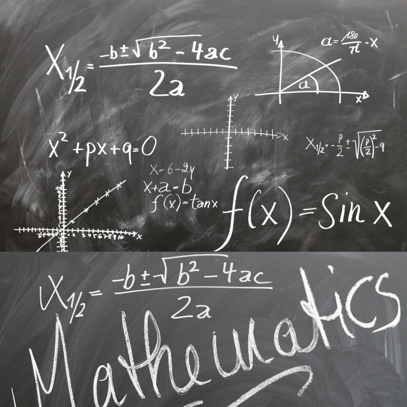
9709 AS Level Mathematics

About Course

Struggling with the jump from IGCSE to AS Level Mathematics? This tutoring program is designed to bridge that gap by identifying your specific learning hurdles and turning them into strengths. We move beyond simple memorization to build a solid logical foundation, ensuring you understand the “why” behind every formula in Pure Maths, Statistics, and Mechanics.

Our lessons focus heavily on past paper mastery and exam technique. We will work side-by-side to break down complex, multi-step questions into simple, manageable parts. With a personalized study plan and consistent timed practice, you will gain the speed and confidence needed to excel on exam day.

Bridging the gap from IGCSE to AS Level
Mastering Pure Maths: Algebra, Functions, and Calculus
Solving Probability, Statistics, and Mechanics problems
Applying formulas to real-world scenarios
Deconstructing past paper exam questions
Structuring logical, step-by-step mathematical proofs
Building speed and accuracy for exam day

Course Content

1. Quadratics
Master the essential bridge between basic algebra and advanced calculus. This course focuses on the core quadratic skills required for AS-Level Mathematics (9709), ensuring you have the precision and logic needed for exam success.Core Syllabus CoverageSolving Equations: Advanced factorization, completing the square, and the quadratic formula.The Discriminant ($b^2 - 4ac$): Determining the number of roots and solving problems involving tangency (where a line meets a curve).Quadratic Functions: Sketching parabolas, identifying the vertex (turning point) through completing the square, and finding intercepts.Inequalities: Solving and sketching regions for $ax^2 + bx + c > 0$ and $ax^2 + bx + c < 0$.Hidden Quadratics: Recognizing and solving equations in other forms (e.g., $x^4$ or substitution-based problems).

QUADRATICS ASSINMENT 1
Quadratic notes

2. Inequalities and Simultaneous Equations
This module focuses on defining and representing ranges of values, moving beyond single-point solutions to understand bounded regions and mathematical constraints.1. Linear InequalitiesAlgebraic Solving: Applying manipulation rules to find the range of values for $x$, including the rule of reversing the inequality sign when multiplying or dividing by a negative number.Graphical Shading: Representing inequalities on a Cartesian plane. You will learn to use dashed lines for "strict" inequalities ($$) and solid lines for "inclusive" inequalities ($leq$ or $geq$).Feasible Regions: Identifying the specific area on a graph that satisfies multiple linear constraints simultaneously.2. Quadratic InequalitiesFinding Critical Values: Determining the roots of a quadratic expression to identify the "boundary points" of the inequality.Parabola Sketching: Using the orientation of the curve (minimum or maximum) to visualize where the function is above or below the x-axis.Solution Sets: Defining whether the solution lies between the two critical values (e.g., $a < x < b$) or in the outer tails (e.g., $x <a> b$).Core Learning ObjectivesTranslation: Converting real-world constraints into mathematical inequality statements.Visualization: Confidently sketching regions to solve problems that are difficult to process through algebra alone.Set Notation: Expressing final answers using formal mathematical notation.

3. Functions
Definition: A rule that maps every input ( ) in the domain to exactly one output ( ) in the range. Key Concepts: Mapping: One-to-one (injective) or many-to-one. Representation: Algebraic formulas ( ), graphs, or mapping diagrams. Types: Linear, Quadratic, Exponential, Trigonometric, and Composite functions. Tools: Vertical Line Test, Domain/Range identification, Inverse functions. Purpose: To model, analyze, and predict relationships between changing quantities

Graphs of Functions
Graphs of FunctionsThis module explores how different algebraic relationships create specific shapes on a coordinate plane, focusing on visual recognition and sketching.1. Polynomial GraphsLinear & Quadratic: Recognizing straight lines and parabolas. You will identify key features like where the graph crosses the axes and the "turning point" (vertex) of a curve.Cubic Functions: Identifying the characteristic "S" shape. Mastery involves finding roots and understanding the general flow of the curve based on the leading term.2. Reciprocal FunctionsCurves & Asymptotes: Learning to sketch graphs like $y = frac{k}{x}$. These curves never touch the axes, creating boundary lines known as asymptotes.Behavior: Understanding how the graph reacts as values get extremely large or extremely close to zero.3. CirclesCenter & Radius: Visualizing circles on a grid. You will learn to identify the center point and the distance to the edge (radius) from the graph's layout.Intersections: Seeing where lines or other shapes cross the boundary of the circle.4. TransformationsShifts: Moving any base graph up, down, left, or right without changing its shape.Reflections: Flipping a graph over the horizontal or vertical axes to create a mirror image.Stretches: Pulling a graph taller or pushing it wider to change its steepness.Core Learning ObjectivesVisual Deduction: Determining the nature of a function just by looking at its shape.Sketching Accuracy: Drawing clear, labeled diagrams that highlight intercepts and stationary points.Relationship Mapping: Understanding how changing a value in a function changes its physical position on a graph.

Combinations of Transformations
When multiple transformations are applied to a single function, the order in which you perform them is the most critical factor. Changing the order can result in an entirely different final graph.1. Vertical CombinationsThese involve shifts, stretches, and reflections that affect the $y$-coordinates. When transformations are applied "outside" the function, follow the standard order of operations.Order: Perform Stretches and Reflections first, then Translations (shifts).Visual Effect: A graph might be stretched vertically and then moved upward. If you move it upward first and then stretch it, the distance it moved is also multiplied by the stretch factor.2. Horizontal CombinationsThese affect the $x$-coordinates and occur "inside" the function. These are often counter-intuitive because they behave in the opposite way to what the notation suggests.Order: Perform Translations (shifts) first, then Stretches and Reflections.Visual Effect: Shifting a graph horizontally before applying a horizontal stretch ensures the shape maintains its new relative position.3. Reflections as FlipsReflections are treated like stretches with a factor of $-1$.Horizontal Reflection: A flip across the vertical axis.Vertical Reflection: A flip across the horizontal axis.When combined with a shift, the "fold line" of the reflection changes depending on whether the shift happened before or after the flip.Key Takeaways for SketchingInside vs. Outside: Always distinguish between changes inside the brackets (affecting $x$) and outside the brackets (affecting y).Step-by-Step Approach: Sketch the base graph first, then apply each transformation one by one to see how the key points (like intercepts or turning points) migrate.Point Mapping: Tracking a single coordinate (x, y)through the sequence of changes is often the most reliable way to ensure accuracy.

Modelling with Functions
This final module focuses on applying your knowledge of graphs and algebra to represent real-world scenarios. Instead of just working with abstract numbers, you will use functions to predict outcomes, find maximum or minimum values, and interpret physical constraints.1. Translating Reality into MathThe first step is identifying which type of function fits a specific situation.Linear Models: Used for relationships with a constant rate of change, such as a taxi fare with a fixed starting fee plus a cost per kilometer.Quadratic Models: Ideal for projectile motion (like the path of a ball), calculating area, or finding the point where a business achieves maximum profit.Exponential Models: Used for things that grow or decay rapidly, like population growth, the cooling of a cup of coffee, or compound interest.2. Identifying ConstraintsEvery real-world model has limits. These are expressed as inequalities or restricted domains.Physical Limits: For example, time cannot be negative, or a container has a maximum volume.Defining the Scope: You must decide which values of $x$ make sense for the model. A graph might technically go on forever, but the "model" only exists within a specific range.3. Finding the "Sweet Spot" (Optimization)A key goal of modeling is finding the best possible outcome.Turning Points: Using the vertex of a parabola to find the maximum height of an object or the minimum cost of production.Intersection Points: Finding where two models meet, such as the "break-even" point where a company's revenue exactly covers its costs.Core Learning ObjectivesInterpretation: Explaining what features like the y-intercept or the gradient mean in a physical context (e.g., "the starting temperature" or "the speed of the car").Prediction: Using a function to calculate an unknown value—for example, predicting the value of a piece of equipment after five years of use.Evaluation: Recognizing the limitations of a model. You will learn to identify when a mathematical prediction might stop being realistic in the real world.

Basic Trigonometry
This module introduces the study of relationships between the sides and angles of triangles. It moves from basic ratios to understanding how these functions behave as waves.1. Right-Angled TrianglesThe foundation of trigonometry is based on the constant ratios between sides for a given angle.The Three Ratios: Defining Sine, Cosine, and Tangent based on the Opposite, Adjacent, and Hypotenuse sides.Finding Unknowns: Using these ratios to calculate missing side lengths or unknown angles when provided with partial information.Special Angles: Memorizing the exact values for $30°$, $45°$, and $60°$, which are frequently used in advanced calculations.2. The Sine and Cosine RulesFor triangles that do not have a $90°$ angle (non-right-angled), these rules allow you to solve for any side or angle.The Sine Rule: Used when you have "matching pairs" of an angle and its opposite side.The Cosine Rule: Necessary when you have two sides and the angle between them, or all three side lengths.Area of a Triangle: Calculating area using the formula involving two sides and the sine of the included angle.[Image showing the Sine Rule and Cosine Rule formulas with a labeled triangle]3. Trigonometric GraphsTrigonometry isn't just about triangles; it describes periodic motion. You will learn the shapes of the fundamental wave functions.The Sine Wave: A smooth curve starting at the origin, oscillating between $1$ and $-1$.The Cosine Wave: Similar to the sine wave but starting at its maximum point ($1$).The Tangent Graph: A unique shape featuring vertical asymptotes where the value becomes undefined.[Image comparing the graphs of Sine, Cosine, and Tangent from 0 to 360 degrees]Core Learning ObjectivesUnit Circle Understanding: Visualizing how angles larger than $90°$ (obtuse and reflex) relate back to basic ratios.Identity Mastery: Simplifying expressions using the fundamental relationship between Sine, Cosine, and Tangent.3D Application: Applying trigonometric principles to find lengths and angles within three-dimensional shapes like pyramids and prisms.

Trigonometric Functions
This module shifts from simple triangle calculations to the study of trigonometry as a set of continuous, periodic functions. You will explore how these ratios behave over an infinite range of angles.1. The Sine and Cosine WavesThese functions represent smooth, repeating oscillations. They are used to model everything from sound waves to tide levels.Periodicity: Understanding that these graphs repeat their shape every $360°$ (or $2pi$ radians).Amplitude: Measuring the height of the wave from its center line to its peak.Key Coordinates: Identifying where the waves hit their maximum, minimum, and zero points.Shutterstock2. The Tangent FunctionThe tangent graph is distinct because it is not a continuous wave; it consists of separate branches.Asymptotes: Identifying the vertical lines where the function is undefined (e.g., at $90°$ and $270°$).Steepness: Observing how the graph approaches infinity as it nears an asymptote.3. Transformations of Trig FunctionsJust like other graphs, trigonometric functions can be shifted and stretched to fit specific data.Vertical Shifts: Moving the entire wave up or down.Frequency Changes: "Squashing" or "stretching" the wave horizontally to change how many cycles occur within a specific range.Phase Shifts: Sliding the wave left or right along the horizontal axis.4. Trigonometric IdentitiesThese are mathematical truths that allow you to simplify complex expressions or solve equations by swapping one form for another.The Tangent Identity: Understanding the relationship between Sine, Cosine, and Tangent.The Pythagorean Identity: A fundamental rule relating the square of Sine and Cosine that equals one.Core Learning ObjectivesEquation Solving: Finding all possible angles that satisfy a specific value (e.g., finding all values of x where sin(x) = 0.5.Symmetry: Using the unit circle or graph symmetry to find related angles in different quadrants.Modeling: Creating a trigonometric function to represent a real-world periodic event, like the height of a ferris wheel over time.

Circular Measure (Radians)
This module introduces radians, an alternative way of measuring angles based on the properties of a circle rather than the arbitrary 360 degrees.1. Understanding RadiansA radian is the angle created when the arc length of a circle is equal to its radius.The Relationship: Since a full circle has a circumference of $2pi r$, there are exactly $2pi$ radians in a full turn ($360^circ$).Conversion: Learning to switch between degrees and radians fluently—where $pi$ radians is equivalent to $180^circ$.2. Arc LengthUsing radians simplifies the calculation of distances along the edge of a circle.Direct Proportion: When the angle is in radians, the arc length is simply the radius multiplied by the angle.Applications: Calculating the distance traveled by a point on a rotating wheel or the length of a pendulum swing.3. Area of a SectorA sector is a "pizza slice" of a circle. Radians provide a more direct way to calculate its surface area.Fraction of a Circle: The area is calculated as a fraction of the total circular area, scaled by the angle in radians.Segments: Learning to find the area of a segment (the region between a chord and an arc) by subtracting the area of a triangle from the area of the sector.Core Learning ObjectivesExact Values: Working with multiples of $pi$ (like $frac{pi}{6}$ or $frac{pi}{4}$) to maintain total accuracy in calculations without rounding decimals.Small Angle Approximations: Understanding how sine, cosine, and tangent behave when angles in radians are very close to zero.Problem Solving: Solving complex geometry problems involving overlapping circles, belts, and pulleys.

Trigonomic Equations

Differentiation

Applications of Differentiation

Equation of a Straight Line

Circles

Binomial Expansion

Arithmetic Progression

Geometric Progressions

Sequences and series

Integration

Further Intergration

Student Ratings & Reviews

No Review Yet

About Course

What Will You Learn?

Course Content

QUADRATICS ASSINMENT 1

Quadratic notes

Notes

Functions

Notes

Notes

Notes

Notes

Notes

Trigonomic Equations

Differentiation

Applications of Differentiation

Equation of a Straight Line

Circles

Binomial Expansion

Arithmetic Progression

Geometric Progressions

Sequences and series

Integration

Further Intergration

Company

Quick Links

Newsletter